Project 4 - Neural Radiance Fields Leia

Part 0.1: Calibrating Your Camera

I captured two sets of image pairs with projective transformations by fixing the center of projection and rotating the camera. Each pair has 40-70% overlap for robust registration.

Part 0.2: Capturing a 3D Object Scan (Lafufu)

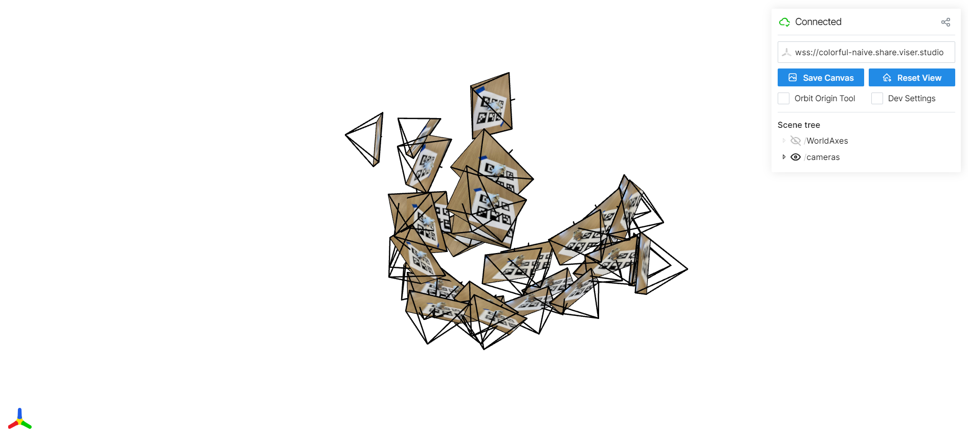
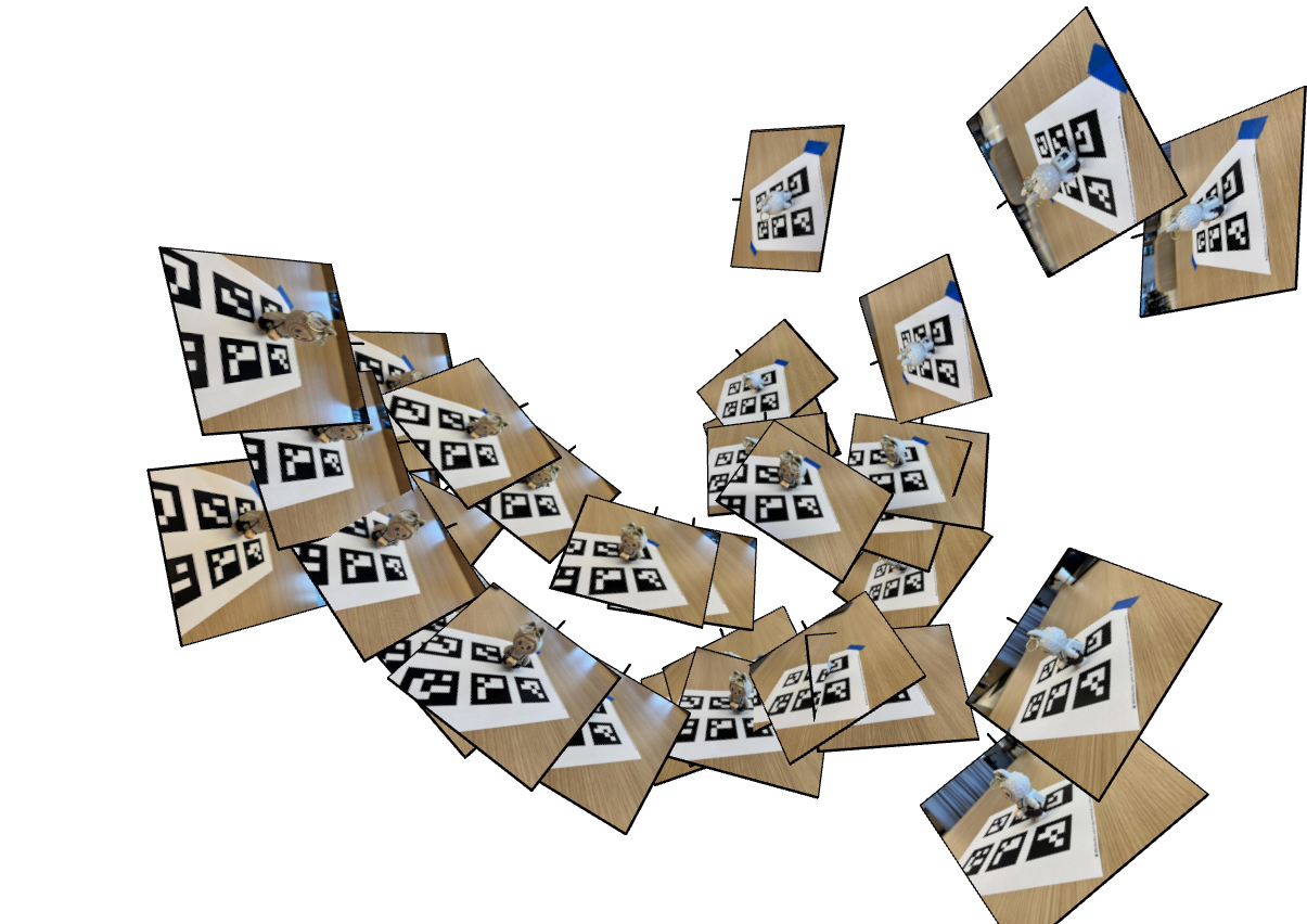
Part 0.3: Estimating Camera Pose

Fixed COP, handheld rotation (~60% overlap). Hearst Mining Building facade.

Part 0.4: Undistorting images and creating a dataset

Fixed COP, handheld rotation (~60% overlap). Hearst Mining Building facade.

Part 2.1: Creating Rays from Cameras

For each training image I convert camera intrinsics and extrinsics into a dense grid of rays. A ray is defined by an origin o (camera center in world space) and a direction d (unprojected pixel through the camera). This lets the network operate directly in 3D, independent of image resolution.

# get_rays: K is intrinsics, c2w is camera-to-world transform
def get_rays(H, W, K, c2w):
    i, j = torch.meshgrid(
        torch.arange(W, device=K.device),
        torch.arange(H, device=K.device),
        indexing="xy",
    )
    pixels = torch.stack([(i - K[0, 2]) / K[0, 0],
                          (j - K[1, 2]) / K[1, 1],
                          torch.ones_like(i)], dim=-1)  # (H, W, 3)

    # Rotate into world space and normalize
    dirs = (pixels[..., None, :] @ c2w[:3, :3].T)[..., 0]
    dirs = dirs / torch.norm(dirs, dim=-1, keepdim=True)

    # Same origin for all pixels: camera center in world coords
    origins = c2w[:3, 3].expand_as(dirs)
    return origins, dirs

Each pixel now corresponds to a ray in world space. These rays drive all later steps: sampling points along them, querying the NeRF network, and volume rendering back into pixel colors.

Part 2.2: Sampling Points Along Rays

Along each ray I sample N=64 points between near and far bounds (t ∈ [2.0, 6.0]). The sampling is stratified: I divide the interval into equal bins and jitter a single sample inside each bin. This reduces aliasing and gives smoother reconstructions.

def sample_points(rays_o, rays_d, N_samples, near=2.0, far=6.0):
    R = rays_o.shape[0]
    t_vals = torch.linspace(near, far, N_samples, device=rays_o.device)  # (N,)
    # Stratified jitter within each bin
    mids = 0.5 * (t_vals[:-1] + t_vals[1:])
    upper = torch.cat([mids, t_vals[-1:]], dim=0)
    lower = torch.cat([t_vals[:1], mids], dim=0)
    t_rand = torch.rand((R, N_samples, 1), device=rays_o.device)
    t = (lower[None, :, None] + (upper - lower)[None, :, None] * t_rand)
    # 3D positions along the ray
    pts = rays_o[:, None, :] + rays_d[:, None, :] * t
    step_size = (far - near) / N_samples
    return pts, t, step_size

Sampling points turns each ray into a small 1D volume. The NeRF network predicts color and density at these points, which we then integrate with volume rendering.

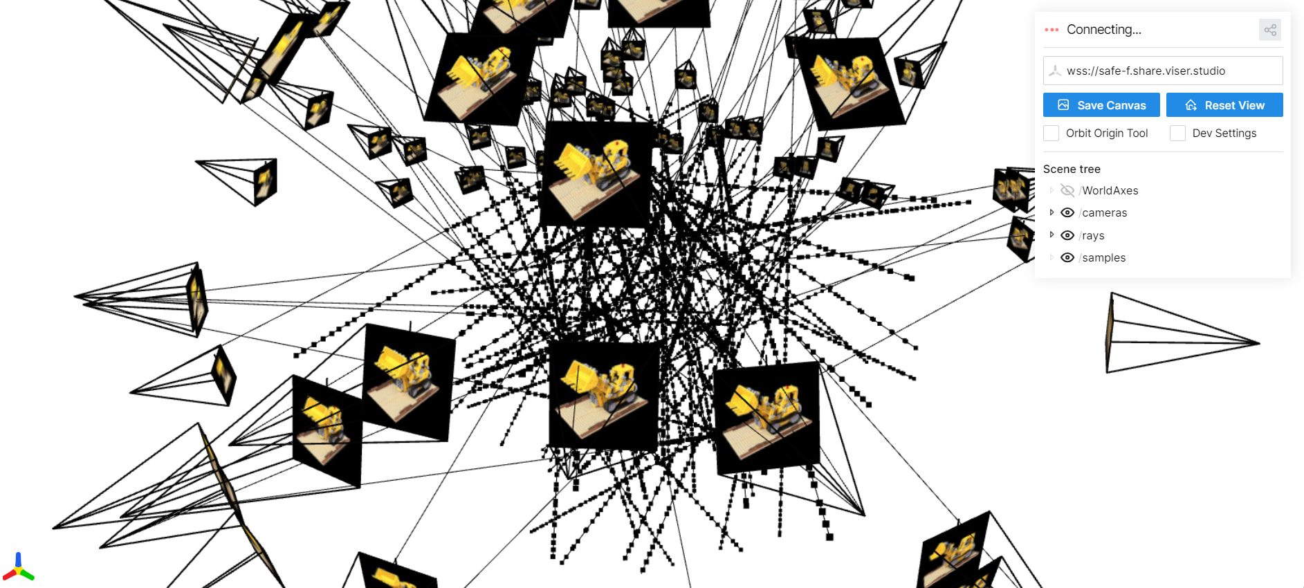
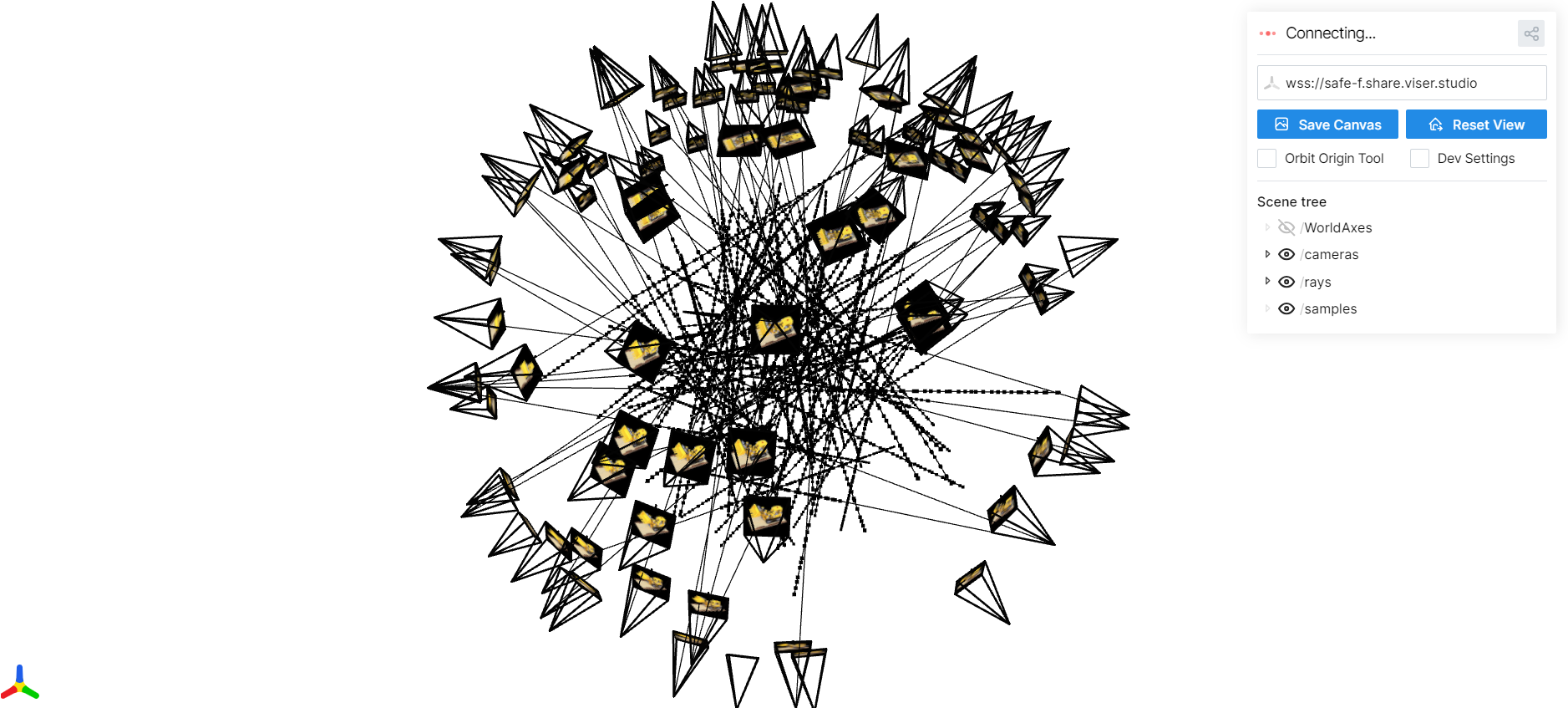
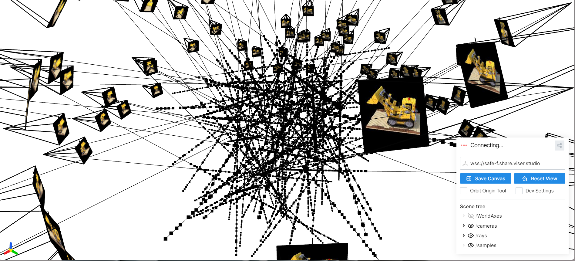
Part 2.3: Visualizing Cameras, Rays, and Samples

Here I visualize the camera frustums, a subset of rays, and the sampled points used to train the NeRF on the Lego scene.

Part 2.4: NeRF Network Architecture

Here I visualize the NeRF MLP that takes in positional encodings of 3D points (and viewing directions) and predicts density and RGB color. The architecture uses several fully connected layers with ReLU activations and skip connections.

Part 2.5: Volume Rendering

Given per-point densities σᵢ and colors cᵢ along each ray, I implement the discrete volume rendering equation in PyTorch. The key idea is to treat the ray as a semi-transparent volume and compute how much light is absorbed and emitted at each step.

def volrend(sigmas, rgbs, step_size):
    """
    sigmas: (B, N, 1) densities along each ray
    rgbs:   (B, N, 3) colors at those samples
    step_size: scalar distance between samples
    returns: (B, 3) rendered colors
    """
    sigma_delta = sigmas * step_size                 # (B, N, 1)
    alphas = 1.0 - torch.exp(-sigma_delta)          # αᵢ = 1 - exp(-σᵢ δ)

    cumsum_sigma_delta = torch.cumsum(sigma_delta, dim=1)
    accum_before = cumsum_sigma_delta - sigma_delta # ∑_{j<i} σⱼ δ

    T = torch.exp(-accum_before)                    # Tᵢ = exp(-∑_{j<i} σⱼ δ)
    weights = T * alphas                            # wᵢ = Tᵢ αᵢ

    return torch.sum(weights * rgbs, dim=1)         # ∑ wᵢ cᵢ

Intuitively, Tᵢ is the probability the ray has not terminated before sample i, and αᵢ is the probability it terminates at i. Their product gives a weight for each sample, and summing the weighted colors yields the final pixel color. This function is fully differentiable and passes the provided assertion test.

Part 2.6: Training NeRF on My Own Captured Object

For this part, I captured my own small scene: a drink placed on a table. I ran COLMAP to recover camera intrinsics and extrinsics, converted them into the NeRF coordinate system, and generated rays exactly as in Parts 2.1–2.3. I trained the same NeRF architecture as before, but tuned a few hyperparameters for this dataset:

• Batch size: 10,000 random rays per iteration
• Samples per ray: 64 stratified samples
• Learning rate: 5e-4 with Adam
• Near / far bounds: 2.0 and 6.0 (chosen to tightly bound the object)

The model is optimized with MSE loss between rendered colors and ground-truth pixels. Below I show the loss curve, some intermediate training renders, and a GIF of a camera circling the object to visualize novel views.

Training Loss

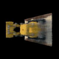
Intermediate Renders During Training

Novel Views: Camera Circling the Object

After training, I rendered a sequence of images by moving a virtual camera in a circular path around the object. These frames are compiled into the GIF below.