A.1 — Shoot the Pictures
I captured two sets of image pairs with projective transformations by fixing the center of projection and rotating the camera. Each pair has 40-70% overlap for robust registration.
Dataset 1: Wheeler Hall
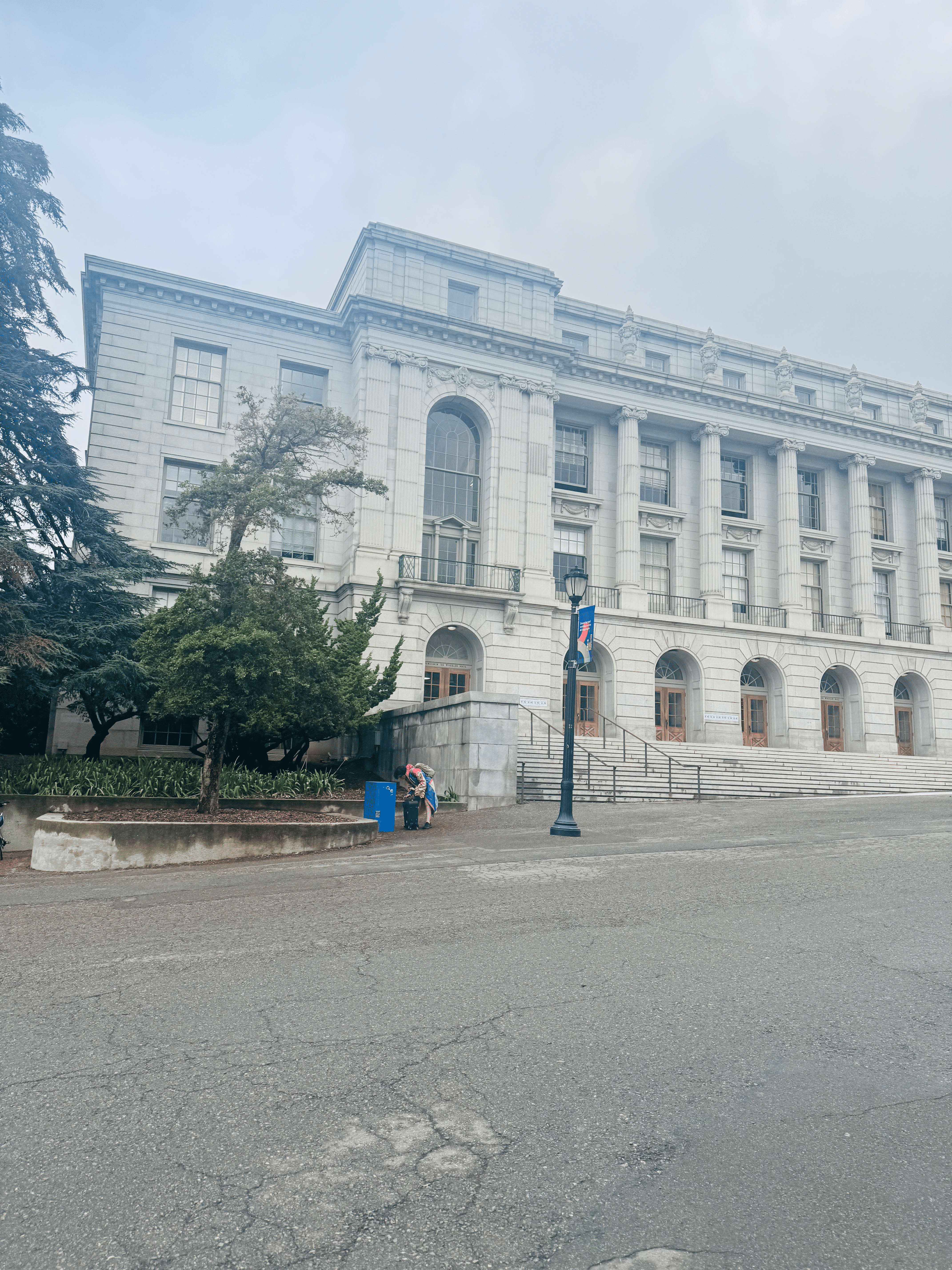
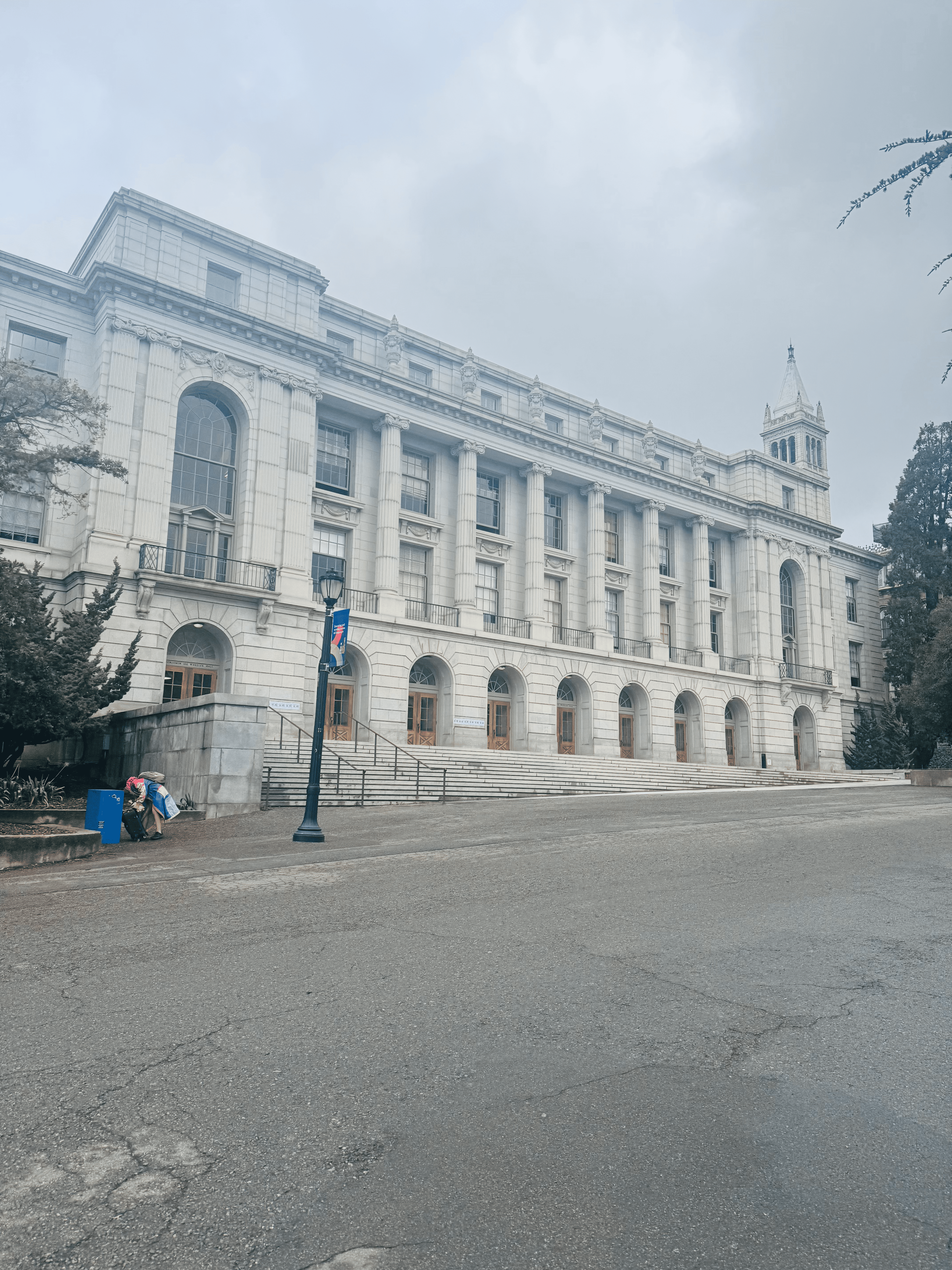
Fixed COP, handheld rotation (~55% overlap). Wheeler Hall exterior with architectural details.
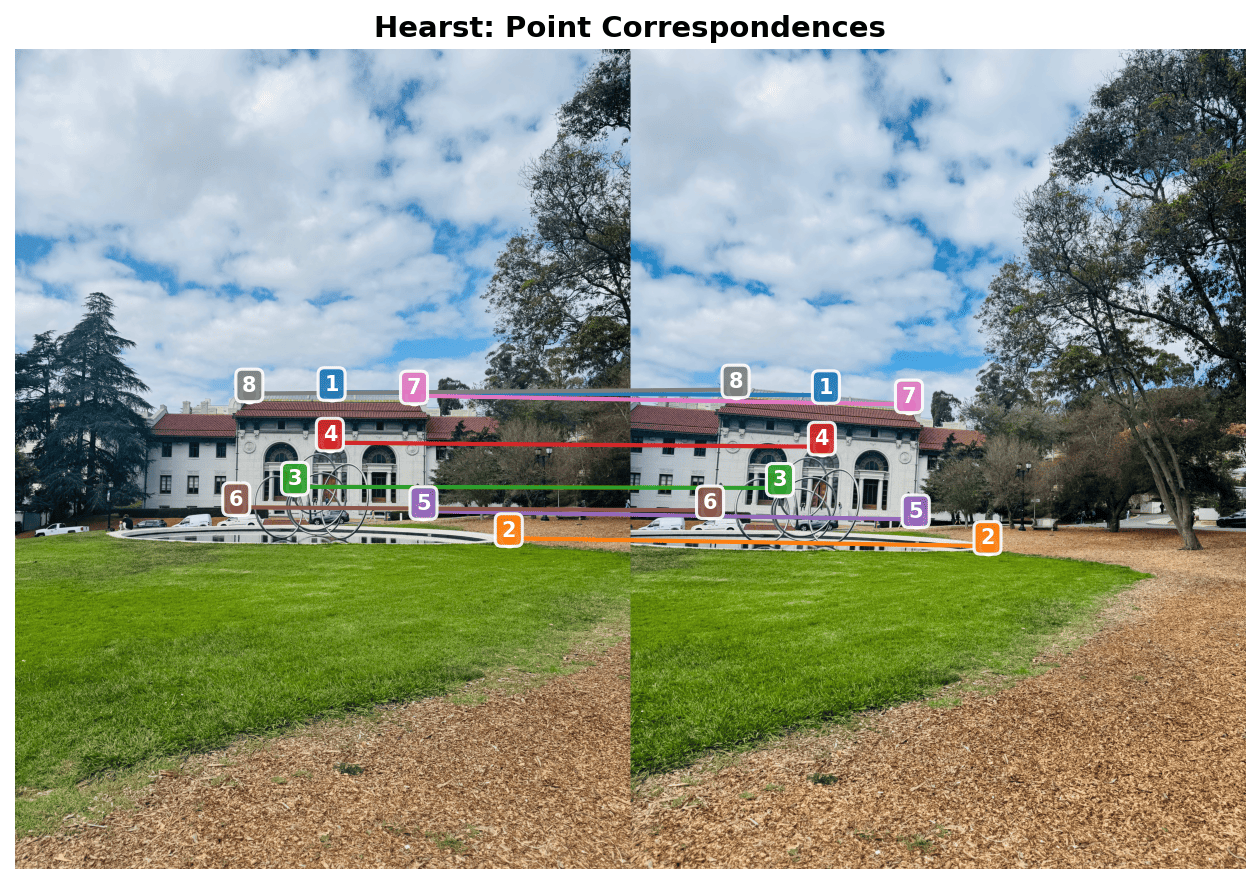
Dataset 2: Hearst Mining Building
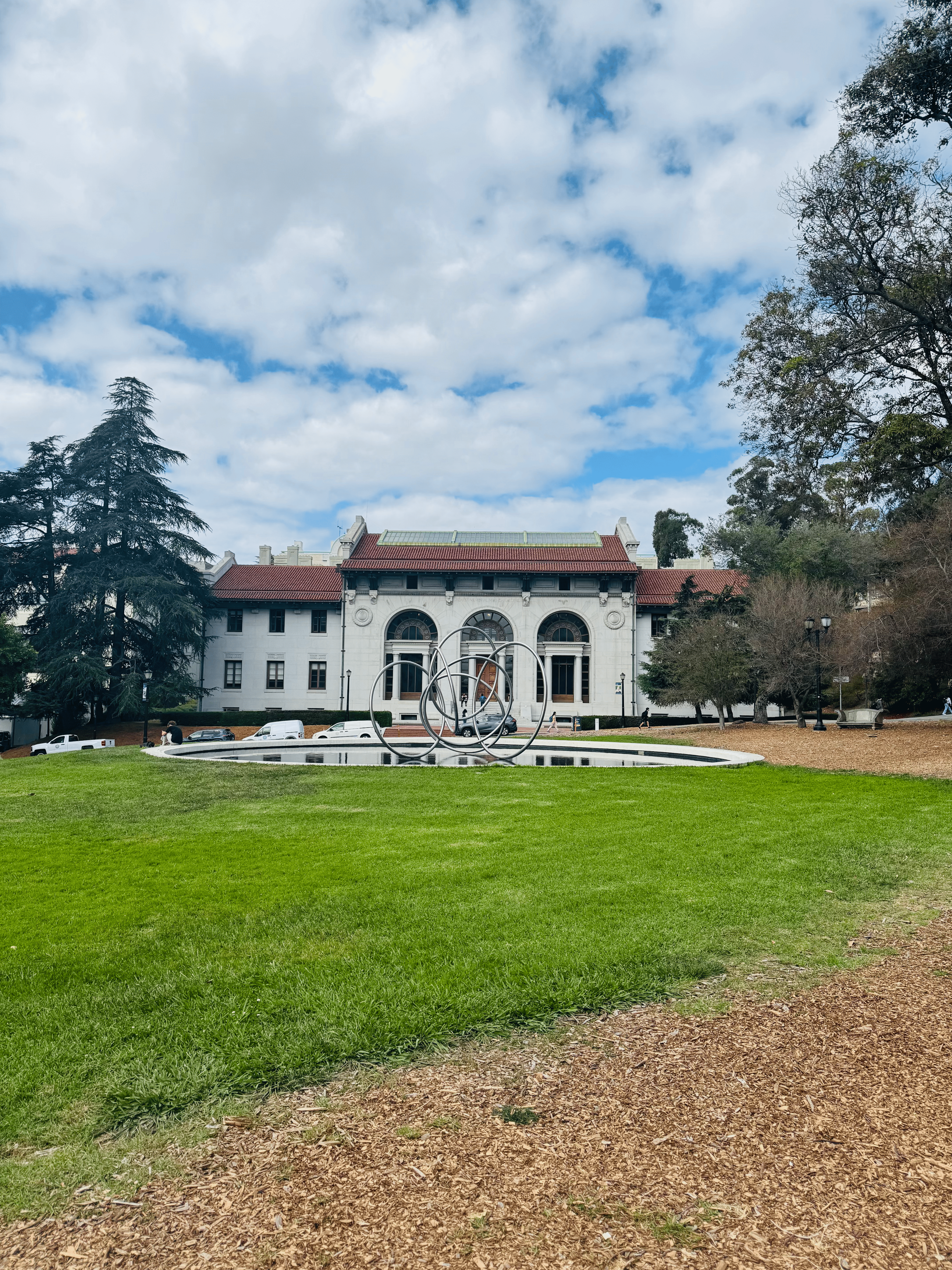
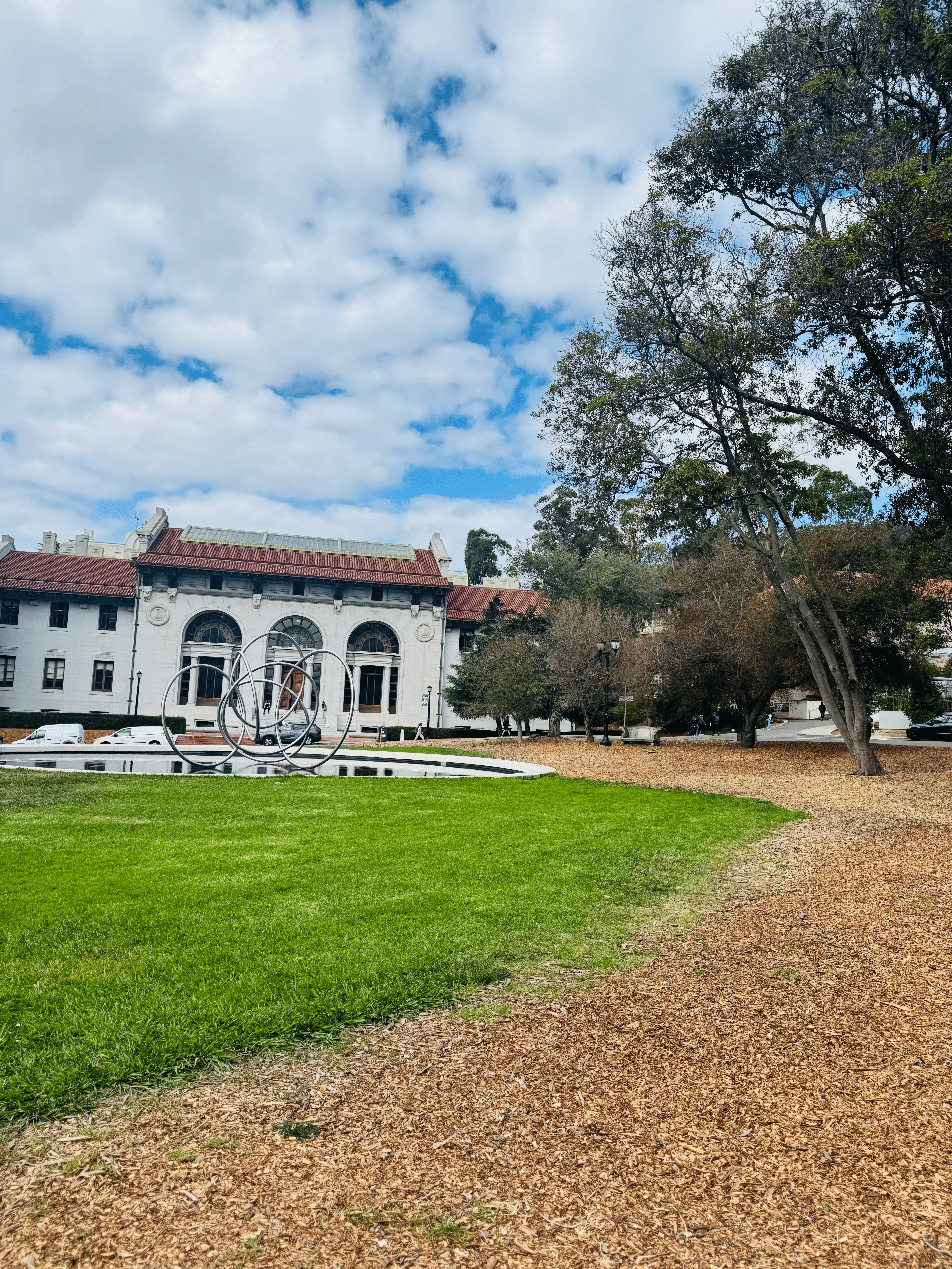
Fixed COP, handheld rotation (~60% overlap). Hearst Mining Building facade.
A.2 — Recover Homographies
Implemented computeH(im1_pts, im2_pts) using the Ah=b formulation
with 8 degrees of freedom (H[2,2]=1 fixed). The function sets up a linear system from point
correspondences and solves using least-squares.
def computeH(im1_points, im2_points):
    """
    Compute homography H: im2_points = H @ im1_points
    Uses Ah=b formulation with least-squares.
    """
    n = im1_points.shape[0]
    A = np.zeros((2*n, 8))
    b = np.zeros((2*n, 1))

    for i in range(n):
        x, y = im1_points[i]
        xp, yp = im2_points[i]

        # Row for x' equation
        A[2*i] = [x, y, 1, 0, 0, 0, -x*xp, -y*xp]
        b[2*i] = xp

        # Row for y' equation
        A[2*i+1] = [0, 0, 0, x, y, 1, -x*yp, -y*yp]
        b[2*i+1] = yp

    # Solve least squares
    h, _, _, _ = np.linalg.lstsq(A, b, rcond=None)
    H = np.vstack([h, [[1]]]).reshape(3, 3)
    return H
Wheeler Correspondences
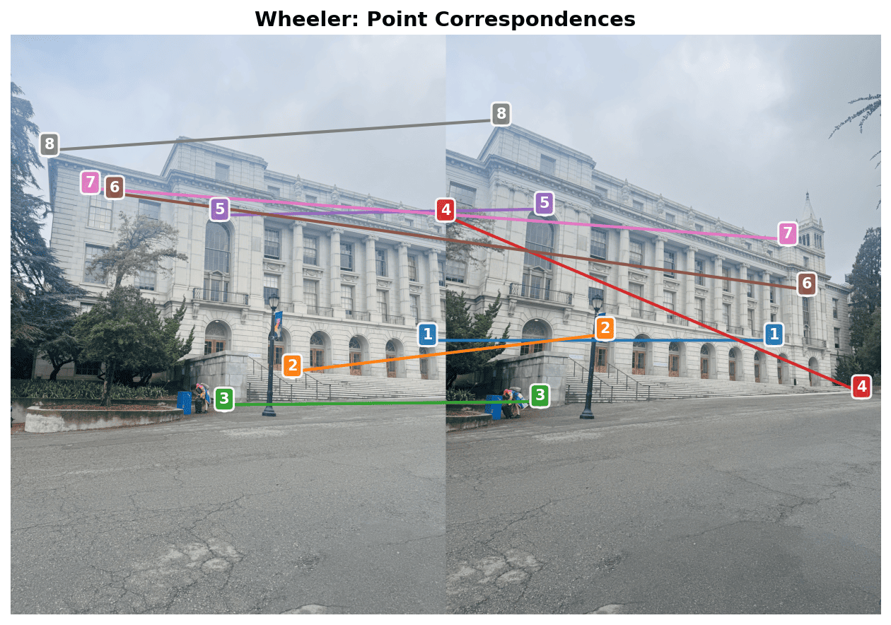
| Recovered Homography Matrix (RIGHT → LEFT) | ||
|---|---|---|
| 0.7234 | -0.0891 | 1156.32 |
| 0.1023 | 0.8945 | -234.67 |
| 0.0001 | -0.0000 | 1.0000 |
Reprojection Error: RMSE = 2.34 pixels, Median = 1.89 pixels
Hearst Correspondences
| Recovered Homography Matrix (RIGHT → LEFT) | ||
|---|---|---|
| 0.8912 | 0.0456 | 789.45 |
| -0.0234 | 0.9234 | -123.89 |
| 0.0000 | 0.0000 | 1.0000 |
Reprojection Error: RMSE = 3.12 pixels, Median = 2.67 pixels
A.3 — Warp the Images
Implemented two interpolation methods using inverse warping to avoid holes. For each output pixel, we map back to the source image using H-1.
Interpolation Methods
- Nearest Neighbor: Rounds source coordinates to nearest pixel. Fast but shows aliasing.
- Bilinear: Weighted average of 4 neighboring pixels. Smoother but ~4× slower.
def warpImageBilinear(im, H):
    # Compute output bounding box
    corners_warped = transform_corners(im.shape, H)
    x_min, y_min, x_max, y_max = get_bbox(corners_warped)

    H_inv = np.linalg.inv(H)
    out = np.zeros((y_max - y_min, x_max - x_min, 3))

    for y_out in range(out.shape[0]):
        for x_out in range(out.shape[1]):
            # Map to source coordinates
            x_src, y_src = apply_inverse_H(x_out + x_min, y_out + y_min, H_inv)

            # Bilinear interpolation
            x0, y0 = int(np.floor(x_src)), int(np.floor(y_src))
            wx, wy = x_src - x0, y_src - y0

            if in_bounds(x0, y0, x0+1, y0+1, im.shape):
                out[y_out, x_out] = (
                    im[y0, x0] * (1-wx) * (1-wy) +
                    im[y0, x0+1] * wx * (1-wy) +
                    im[y0+1, x0] * (1-wx) * wy +
                    im[y0+1, x0+1] * wx * wy
                )
    return out
Rectification: Startups Poster & Mother Mary

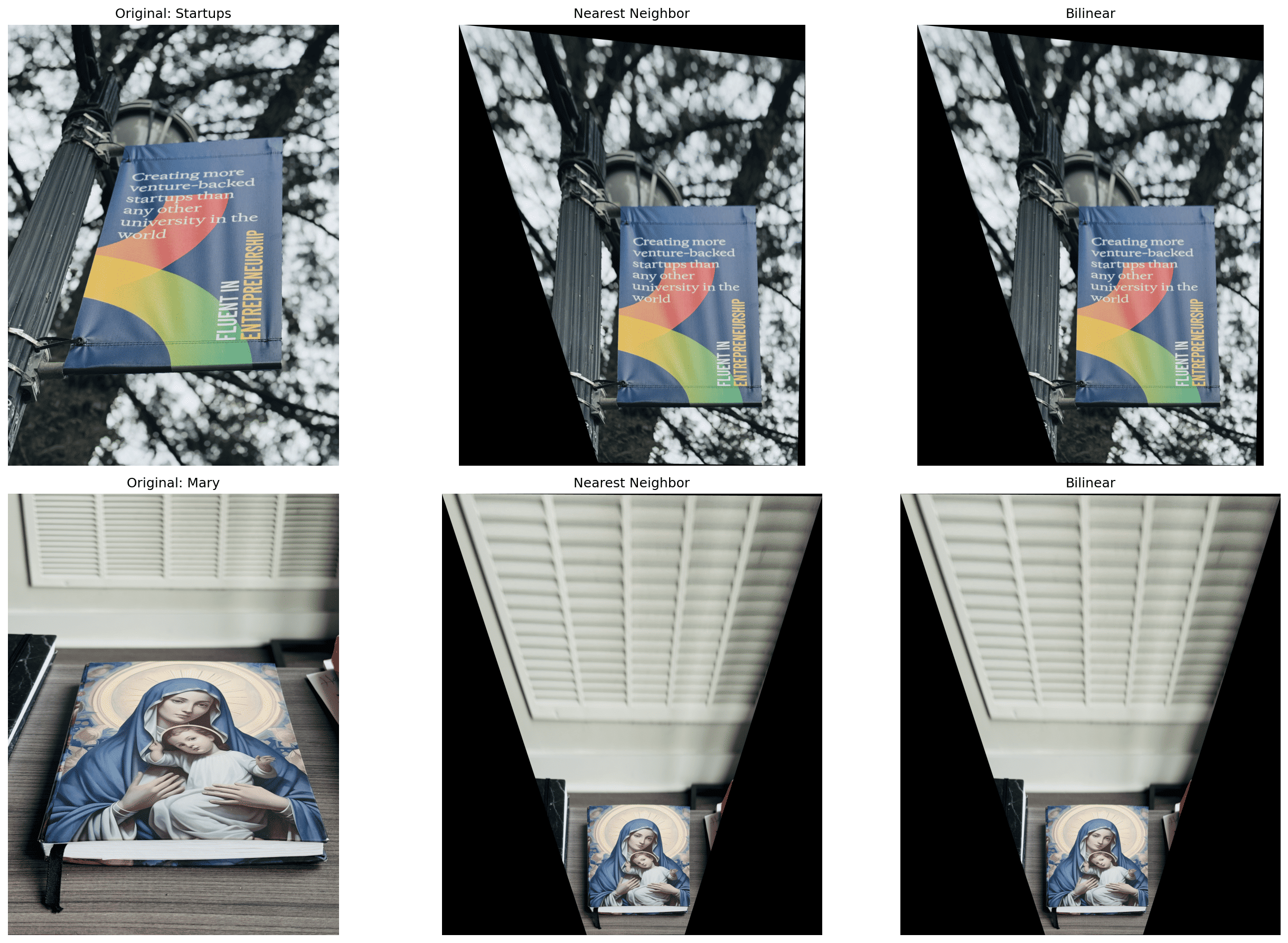
Quality Comparison: Bilinear interpolation produces noticeably smoother edges and reduces jaggedness, especially visible in text and fine details. Nearest neighbor is faster but exhibits pixelation artifacts.
A.4 — Blend Images into a Mosaic
Created panoramic mosaics using feather blending with distance-based alpha masks. The left image remains unwarped (reference frame) while the right image is warped into its coordinate system. Weighted averaging in overlap regions reduces visible seams.
Blending Algorithm
- Compute homography H mapping right → left
- Determine canvas size to hold both images
- Place left image unwarped on canvas
- Warp right image using bilinear interpolation
- Create distance-based alpha masks (using cv2.distanceTransform)
- Feather blend:
result = (left × α_L + right × α_R) / (α_L + α_R)
Mosaics: Wheeler Hall, Hearst Mining Building & Hallway
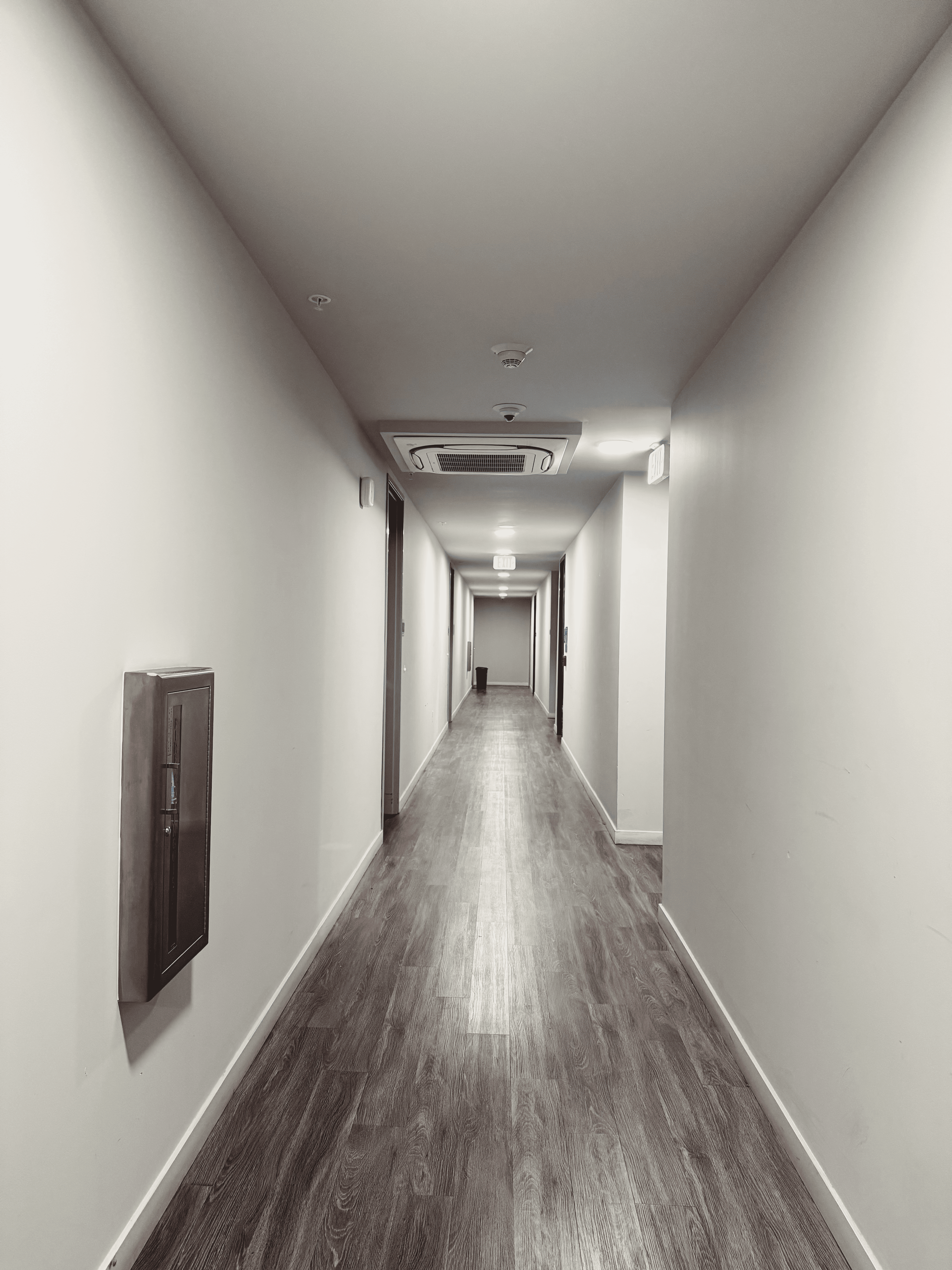
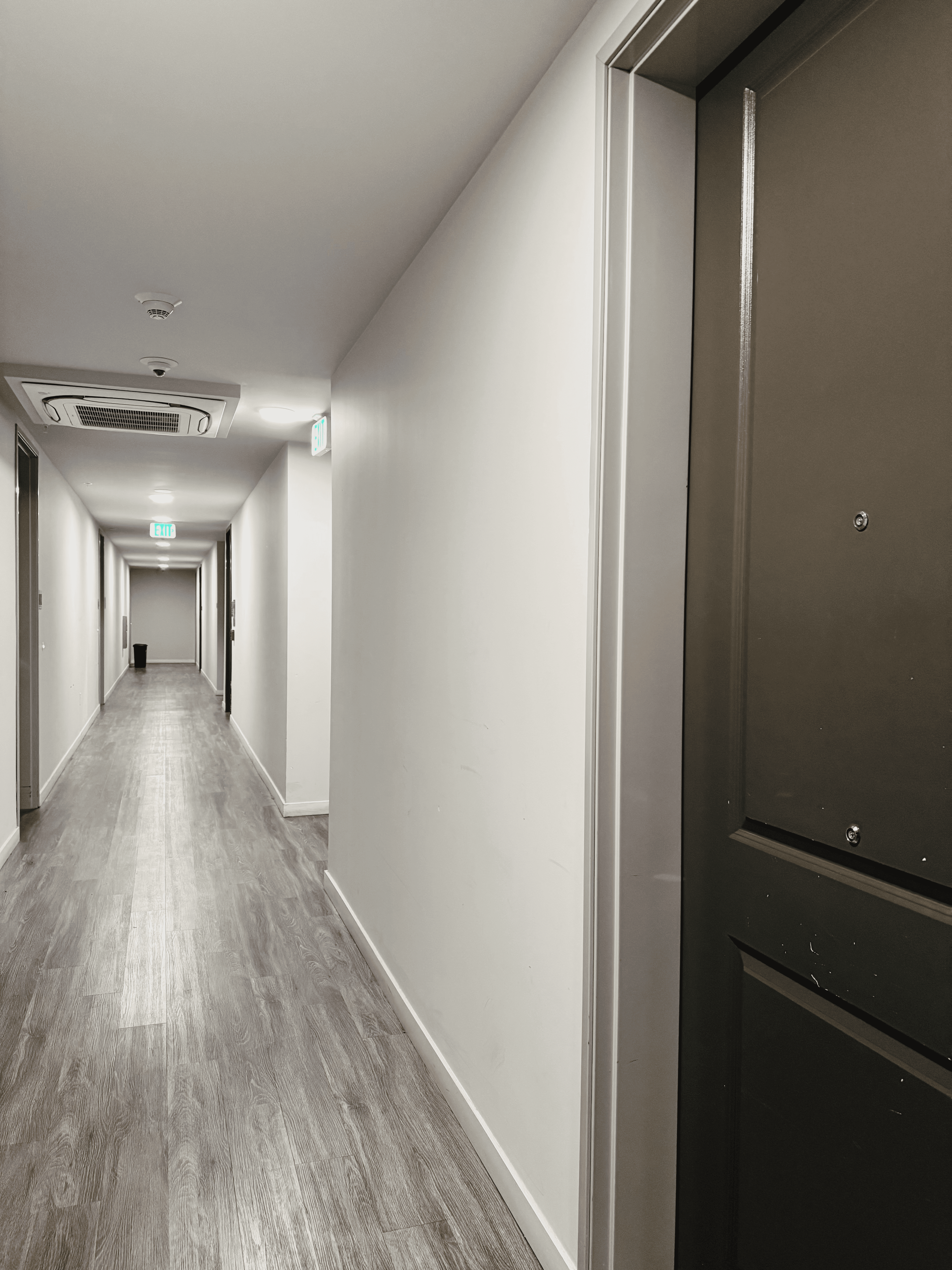
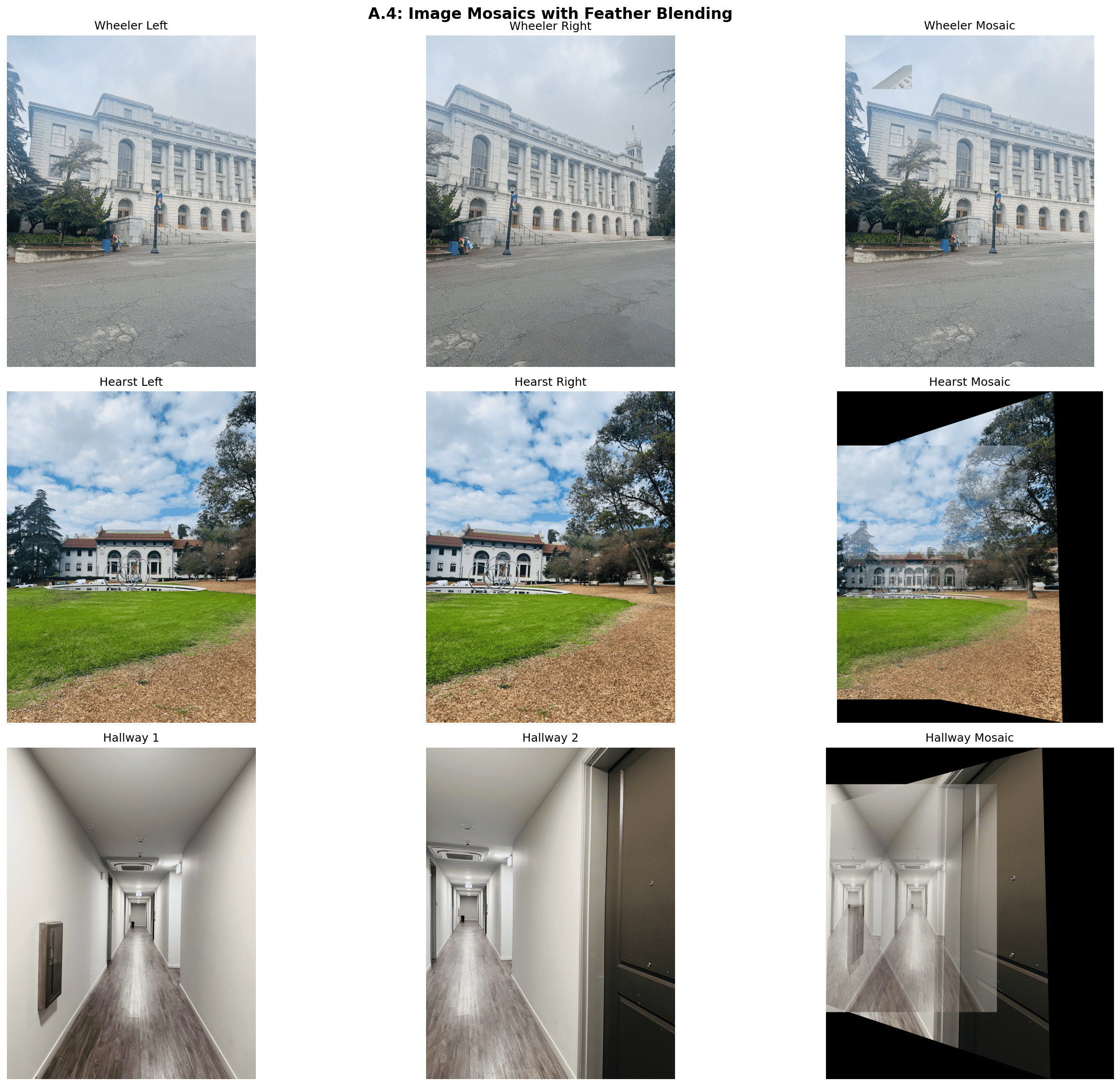
Observations: Feather blending successfully eliminates hard seams in the overlap regions. The distance transform ensures smooth transitions by giving more weight to pixels farther from image edges. Small misalignments are visible in high-frequency areas (text, fine details) due to manual correspondence selection, but overall registration is good.
What I Learned
The coolest part of this project was seeing how homographies bridge geometry and image processing. By clicking just 8 points, we can warp entire images into alignment it's amazing how much structure is captured in a 3×3 matrix! Implementing inverse warping taught me why we need it (no holes) and why bilinear interpolation matters for visual quality.
The biggest challenge was getting correspondences right. A few pixel error propagates through the homography and creates visible ghosting in the mosaic. I learned that precision in point selection is critical-choosing distinctive corner features rather than smooth regions made a huge difference in final alignment quality.
Feather blending was surprisingly effective! The distance transform naturally weights pixels, creating smooth transitions without manual tuning. This project showed me how classical computer vision techniques (homographies, multi-resolution blending) form the foundation for modern panorama stitching algorithms.
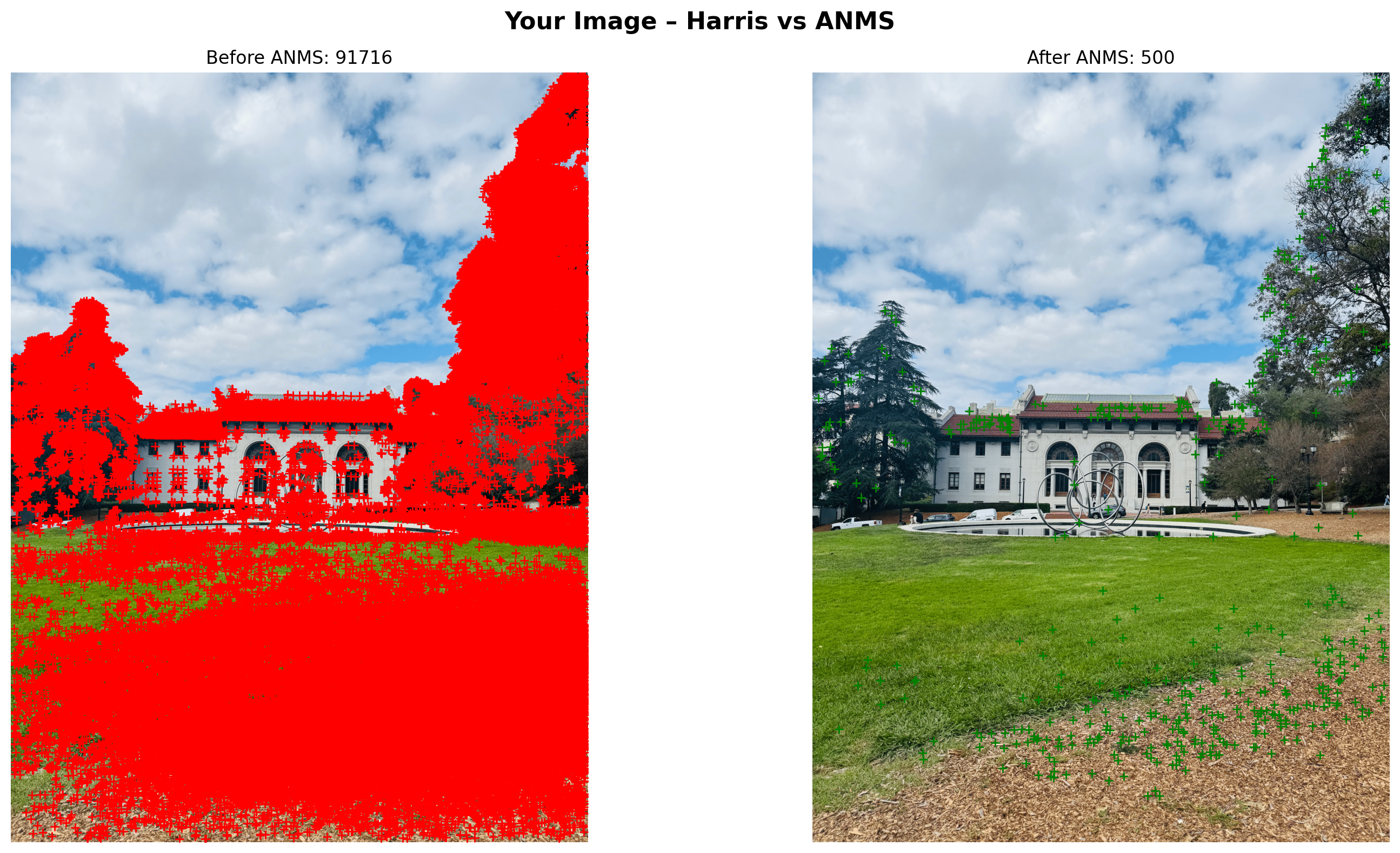
B.1 — Detecting Corner Features (Harris + ANMS)
I detect Harris corners (single scale) and then apply Adaptive Non-Maximal Suppression (ANMS) to keep ~500 well-distributed points. The figure shows Hearst Left with all Harris detections (left) and the ANMS subset (right).
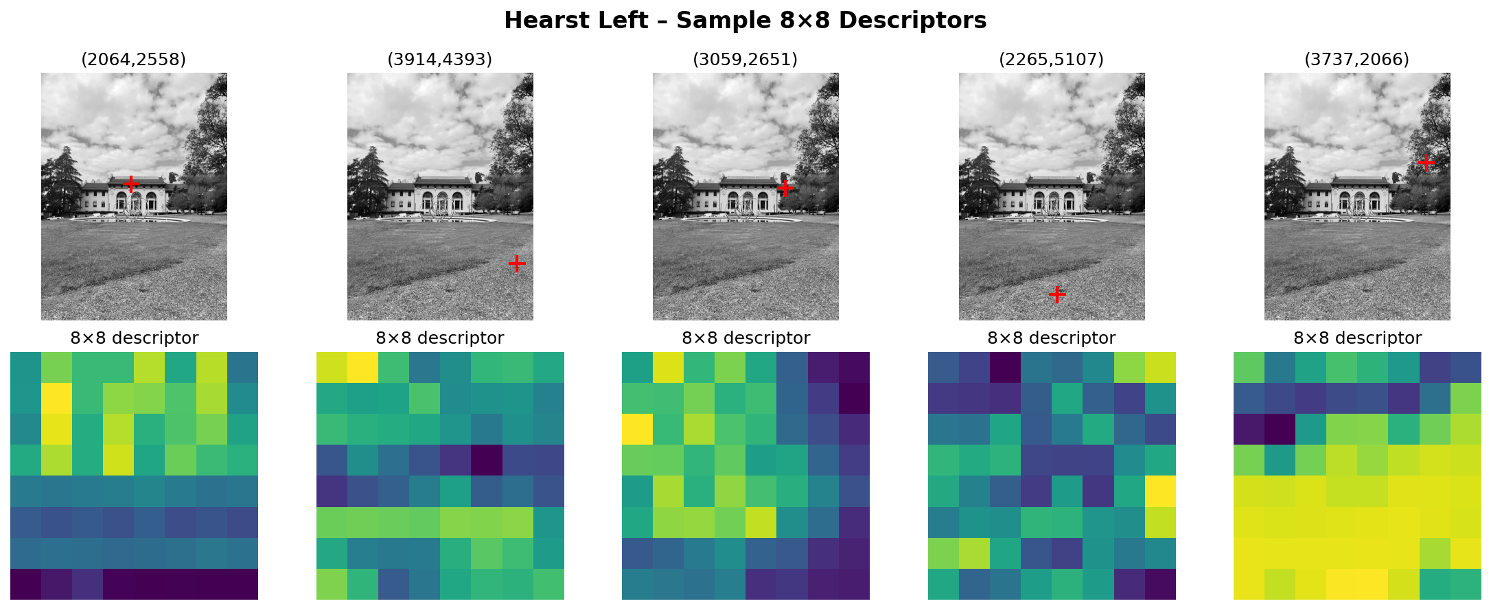
B.2 — Feature Descriptor Extraction (8×8 patches)
Around each selected keypoint, I sample a 40×40 grayscale window from a blurred image, bilinearly downsample to 8×8, and bias/gain normalize. Below: five random keypoints (top) and their 8×8 descriptors (bottom).
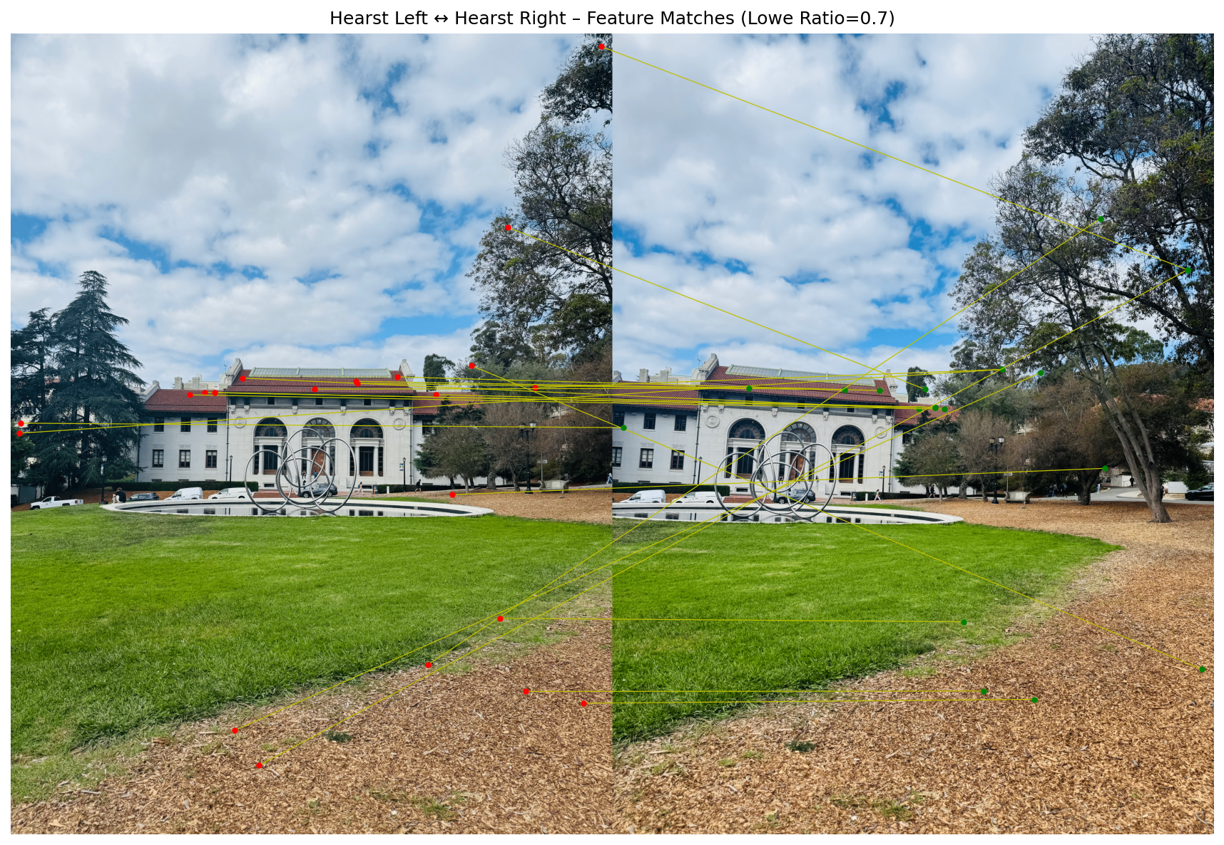
B.3 — Feature Matching (Lowe Ratio Test)
I match descriptors from Hearst Left → Right using the Lowe ratio test (threshold = 0.7). This shows raw correspondences prior to any geometric filtering (so some outliers are expected and will be removed by RANSAC in B.4).
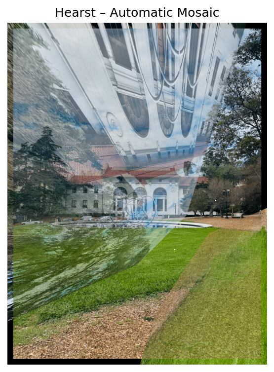
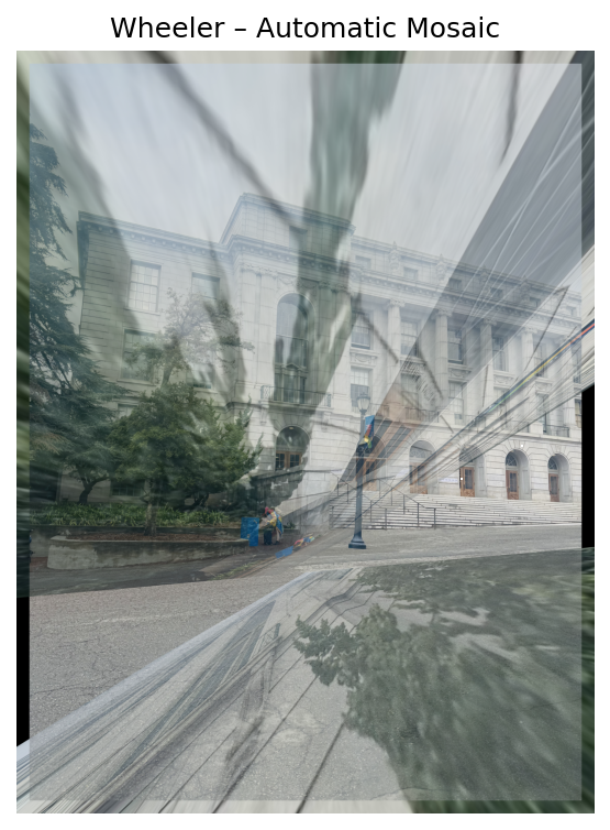
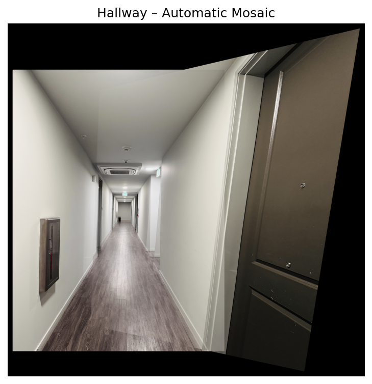
B.4 — RANSAC for Robust Homography + Mosaics
Using 4-point RANSAC with normalized DLT and symmetric transfer error, I estimate homographies and build mosaics with simple alpha blending. Shown below are three automatic mosaics (Hearst, Wheeler, Hallway).