Project 2 – Fun with Filters and Frequencies Leia

Part 1.1 — Convolutions from Scratch

I implemented 2D convolution two ways: a 4-loop version and a faster 2-loop version. Verified against scipy.signal.convolve2d.

# 4-loop conv (numpy only)
def conv2d_naive_4loops(img, kernel):
    img = img.astype(np.float32)
    k = np.array(kernel, np.float32)[::-1, ::-1]  # flip
    H, W = img.shape; kh, kw = k.shape
    ph, pw = kh//2, kw//2
    p = np.pad(img, ((ph, ph), (pw, pw)), mode='constant')
    out = np.zeros((H, W), np.float32)
    for i in range(H):
        for j in range(W):
            acc = 0.0
            for u in range(kh):
                for v in range(kw):
                    acc += p[i+u, j+v] * k[u, v]
            out[i, j] = acc
    return out

# 2-loop conv (vectorized patch)
def conv2d_naive_2loops(img, kernel):
    img = img.astype(np.float32)
    k = np.array(kernel, np.float32)[::-1, ::-1]
    H, W = img.shape; kh, kw = k.shape
    ph, pw = kh//2, kw//2
    p = np.pad(img, ((ph, ph), (pw, pw)), mode='constant')
    out = np.zeros((H, W), np.float32)
    for i in range(H):
        for j in range(W):
            region = p[i:i+kh, j:j+kw]
            out[i, j] = np.sum(region * k)
    return out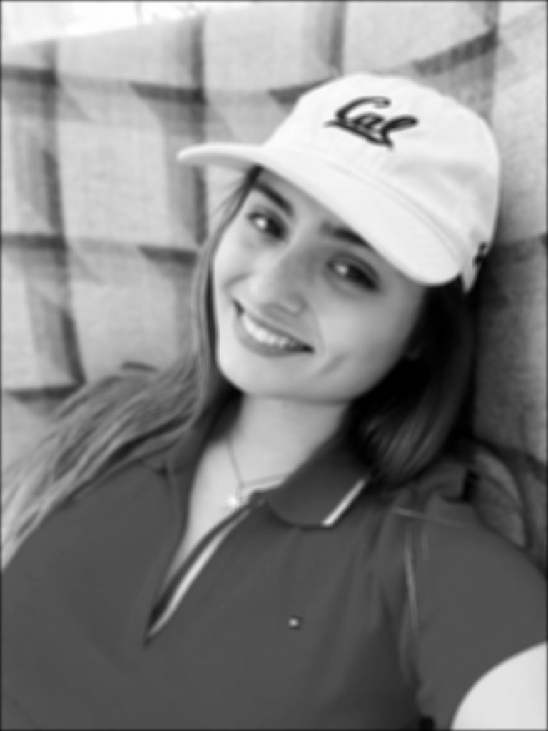

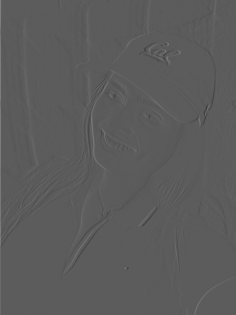
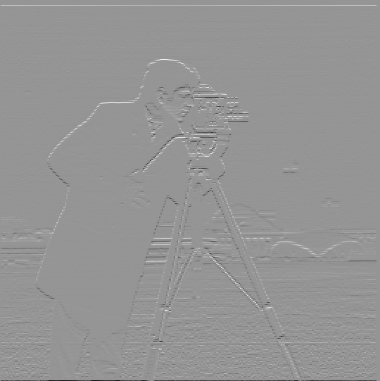
Part 1.2 — Finite Difference Operator

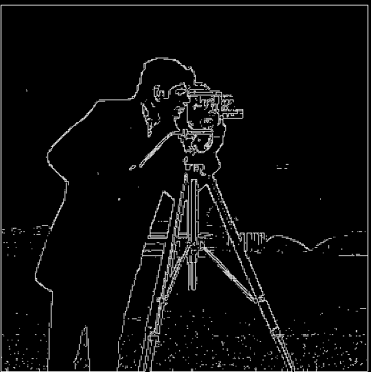
Convolved cameraman with \(D_x=[1,-1]\) and \(D_y=[1\; -1]^T\), then formed \( \sqrt{G_x^2 + G_y^2} \) and thresholded it to make a binary edge map.

# Using convolve2d to compute finite differences
gx = convolve2d(img, np.array([[1,-1]]), mode='same', boundary='symm')
gy = convolve2d(img, np.array([[1],[-1]]), mode='same', boundary='symm')
mag = np.sqrt(gx**2 + gy**2)
edges = (mag > 0.1).astype(np.float32)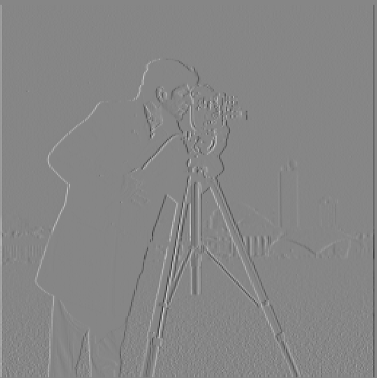

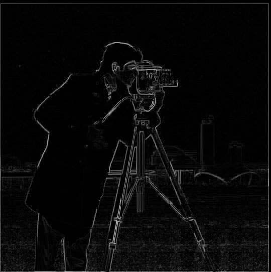
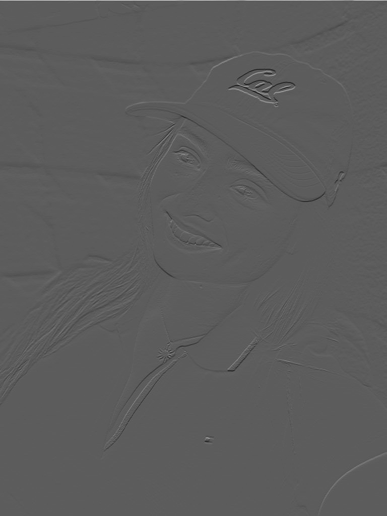
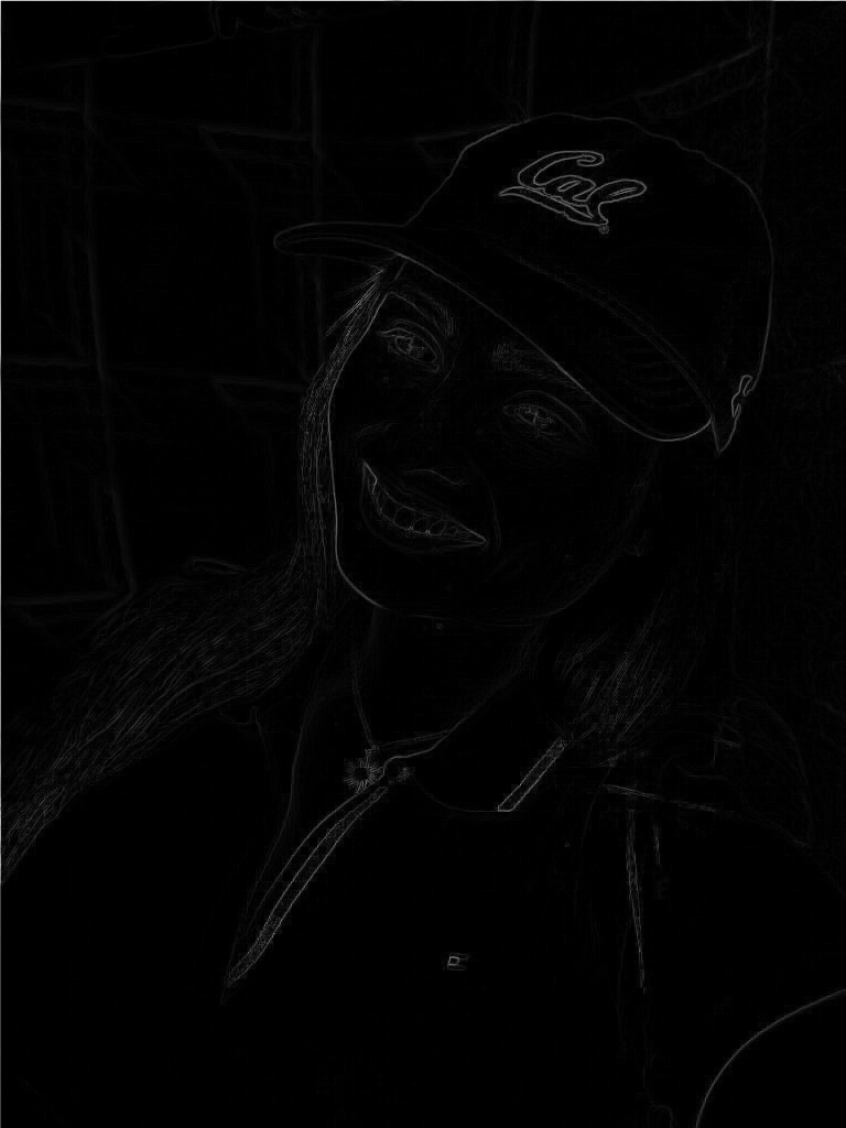
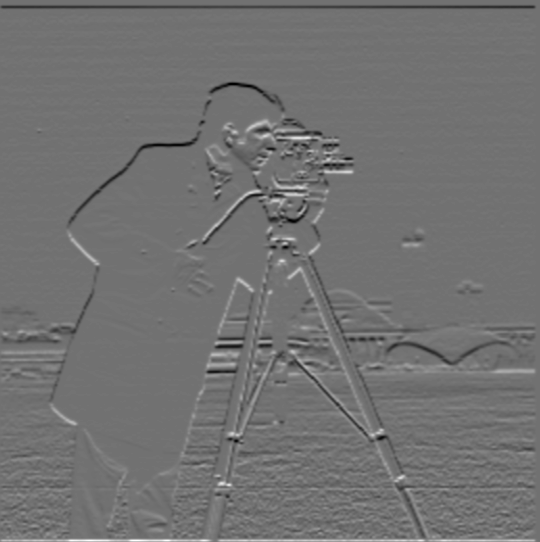
Part 1.3 — Derivative of Gaussian (DoG)

To reduce noise, I smooth with a Gaussian then differentiate (or use DoG kernels). Edges are much cleaner than raw finite differences.

# DoG filter example
g = cv2.getGaussianKernel(ksize=7, sigma=1.5)
gx = -np.arange(-3,4)/1.5**2 * g[:,0]  # derivative part
dogx = convolve2d(img, gx[np.newaxis,:], mode='same', boundary='symm')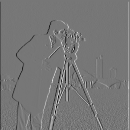

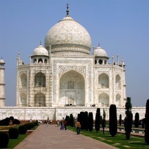
Part 2.1 — Image “Sharpening” (Unsharp Mask)

Unsharp masking: sharpened = image + α × (image − blur).

Taj Mahal

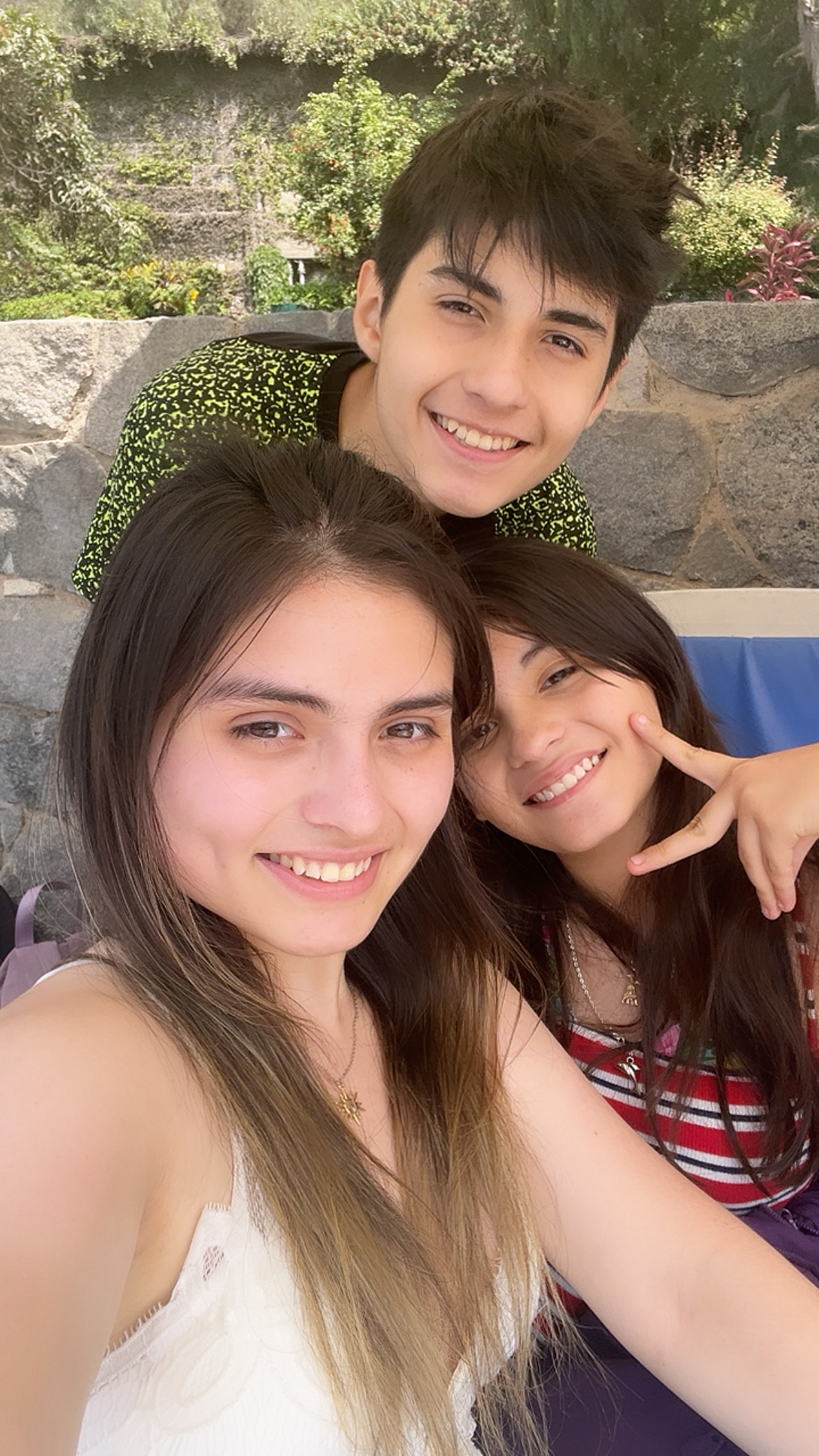
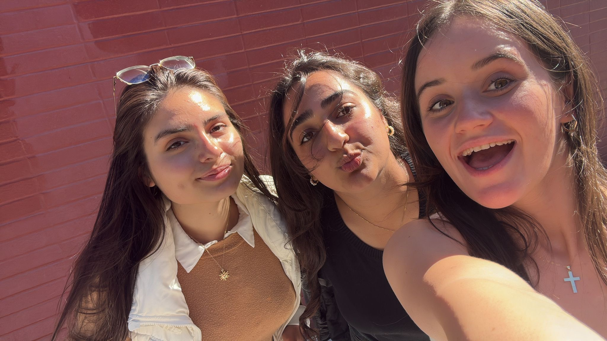
Siblings

Blur → Sharpen Experiment

I picked a sharp image, blurred it, then tried to sharpen it again. Observations: The “recovered” image looks sharper and more detailed than the blurred version, but it cannot fully restore the lost high frequencies. Edges regain contrast but fine textures do not fully come back—showing unsharp masking enhances but does not recreate detail.

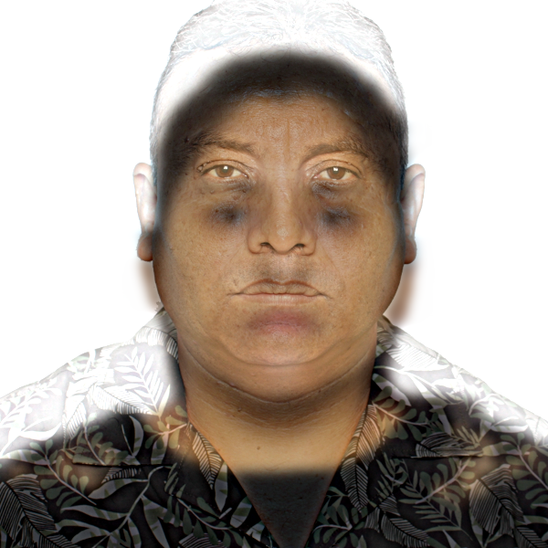
Part 2.2 — Hybrid Images

Low frequencies from one image + high frequencies from another.

Part 2.3 — Gaussian & Laplacian Stacks

I implemented functions gaussian_stack(img, levels, sigma) and laplacian_stack(img, levels, sigma). Gaussian stacks are created by repeatedly blurring the image, while Laplacian stacks are formed by subtracting consecutive Gaussian levels. The last Laplacian level holds the most blurred residual.

def gaussian_stack(img, levels, sigma):
        stack = [img.copy()]
        current = img.copy()
        for i in range(levels - 1):
            current = gaussian_blur(current, sigma)
            stack.append(current.copy())
        return stack
    
    def laplacian_stack(img, levels, sigma):
        gauss_stack = gaussian_stack(img, levels, sigma)
        lap_stack = []
        for i in range(levels - 1):
            lap_stack.append(gauss_stack[i] - gauss_stack[i+1])
        lap_stack.append(gauss_stack[-1])
        return lap_stack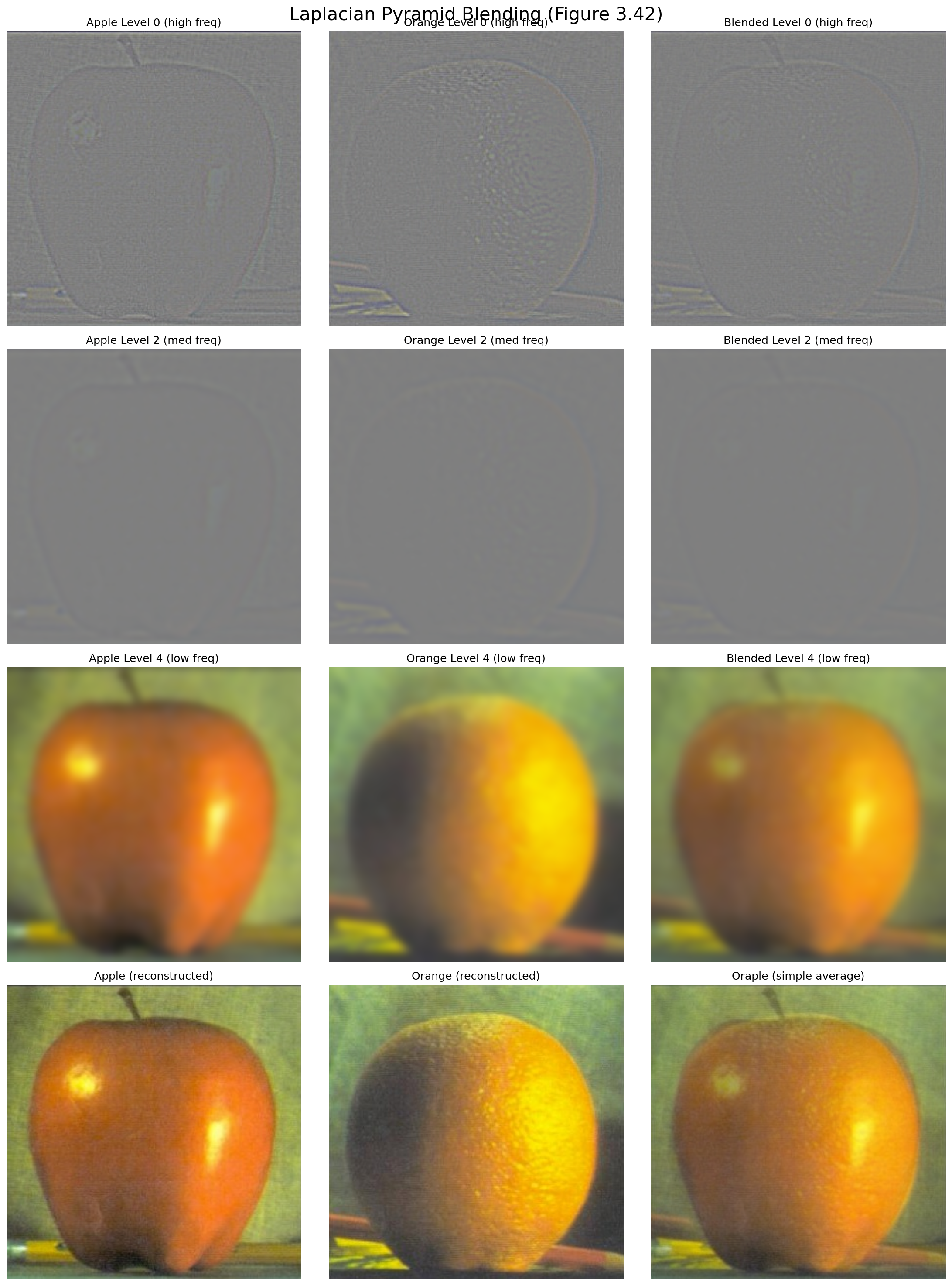

Each Gaussian level is smoother than the last, while each Laplacian level isolates different frequency bands. Summing across all Laplacian levels reconstructs the original image. These stacks are the foundation for the seamless blending in Part 2.4.

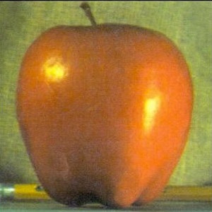
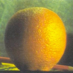
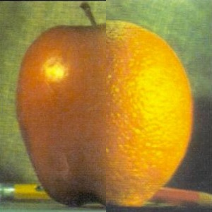
Part 2.4 — Multiresolution Blending

Oraple (Vertical Seam)

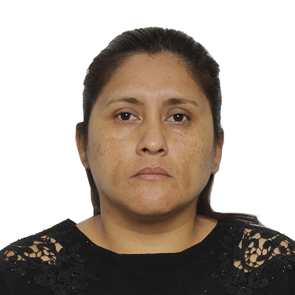
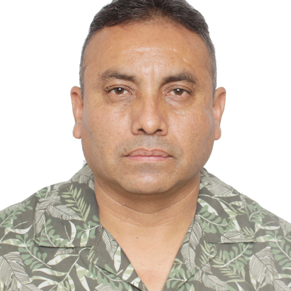
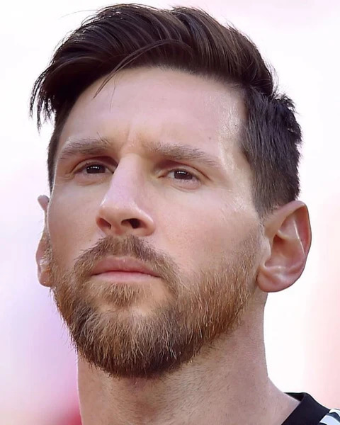
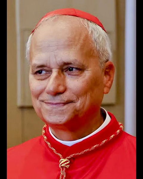
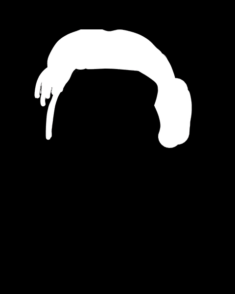
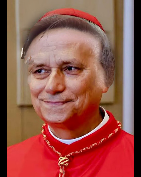
Messi Hair + Pope Face (Irregular Mask)

Cotton Candy Dress (Irregular Mask)

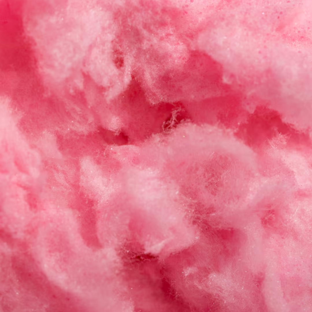
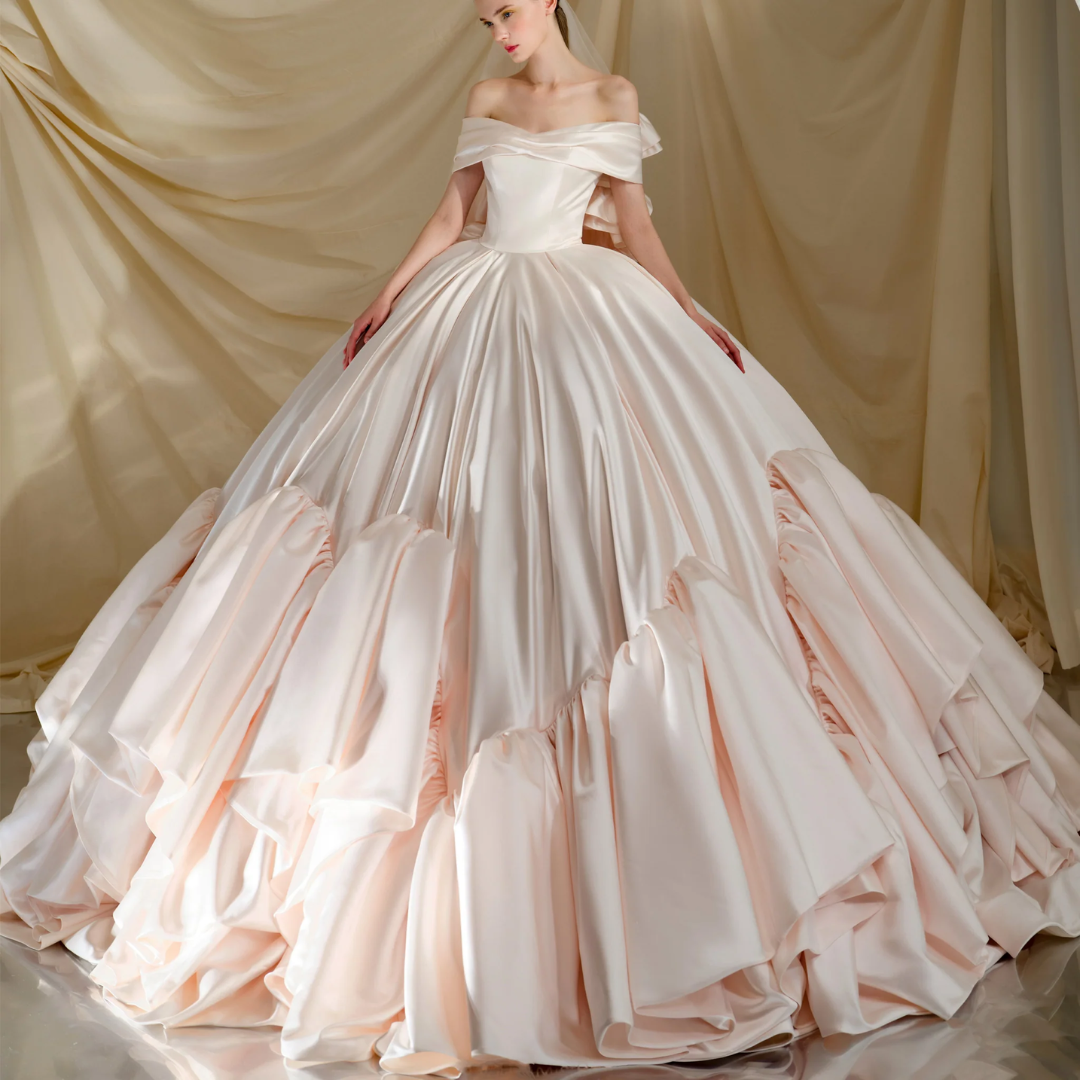
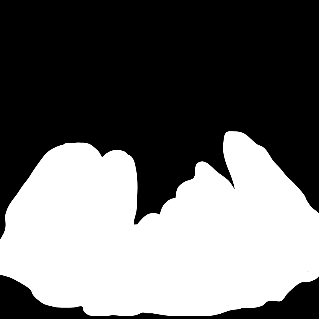
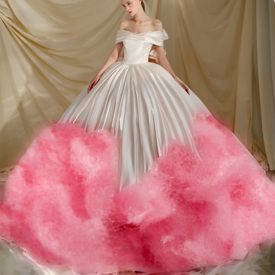
I use Laplacian stacks for each input and a Gaussian stack of the mask. At every level \(i\): blend_i = mask_i · LapA_i + (1 - mask_i) · LapB_i. The final result is the sum over all blended levels. This follows Burt & Adelson’s multiresolution blending and smooths the transition across frequencies (fine detail to coarse structure).